LAB 1: Introduction RStudio and R

BIO3782: Biologist's Toolkit (Dalhousie University)

---

Lab mechanics (how to work through the labs of this course)

For the labs in this course you will need 3 programs:

1. Lab manual: It is a web-page with instructions on what to do in the lab. If you are reading "this", you already found the lab manual. The Lab manual is viewed inside your browser (e.g. Firefox, Chrome, Safari, etc.).
2. Brightspace LAB Questions: In the Lab manual there are several questions that you will need to answer in a corresponding Brightspace LAB Questions. Same as the Lab manual, the Brightspace LAB Questions is viewed inside your browser (e.g. Firefox, Chrome, Safari, etc.). You can get to the Quizzes section in Brightspace following Assessment > Quizzes
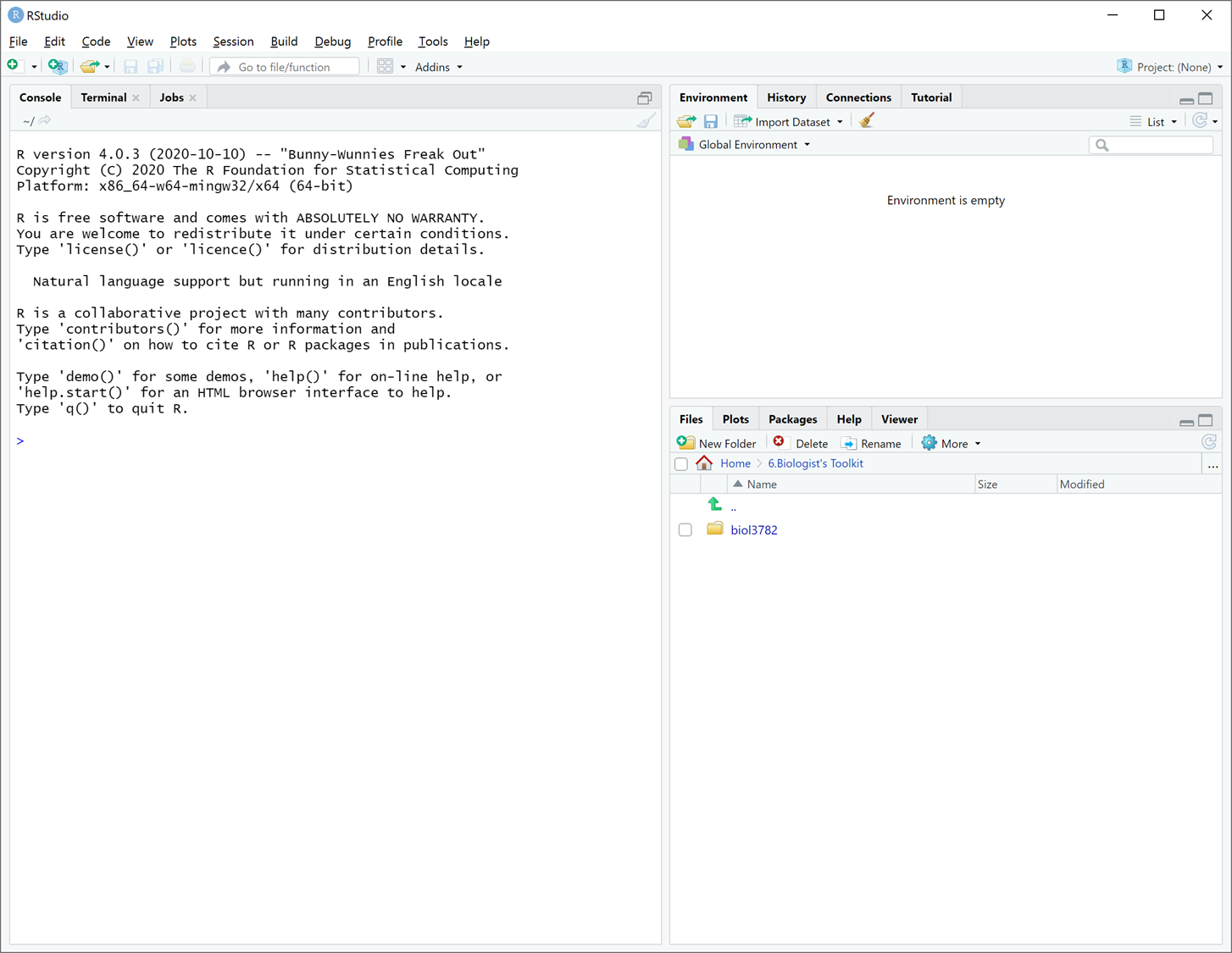
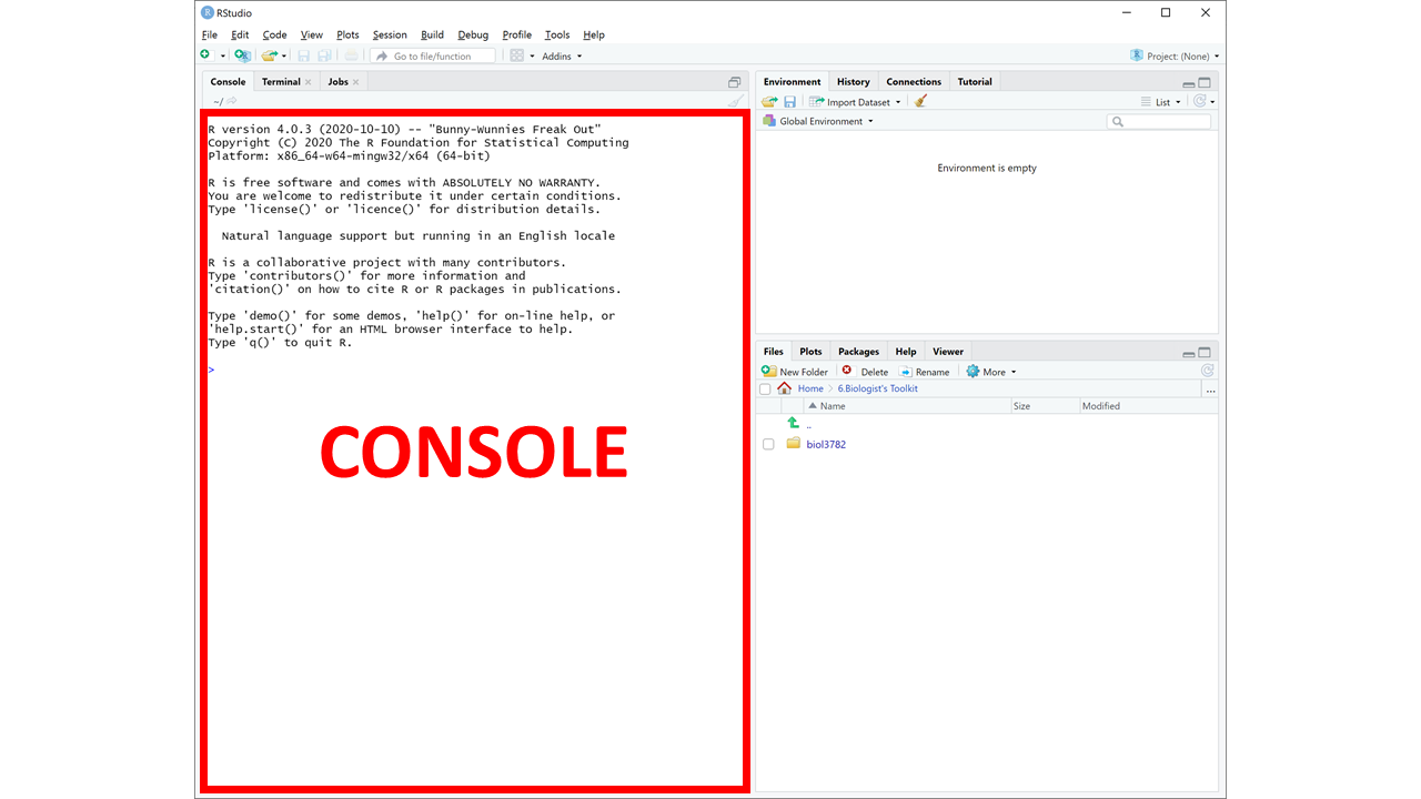
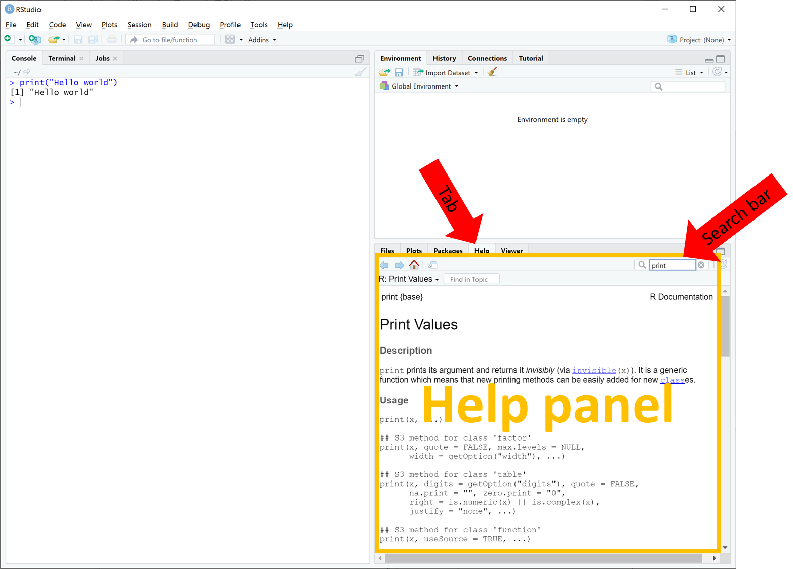
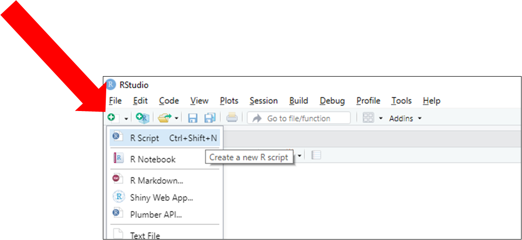
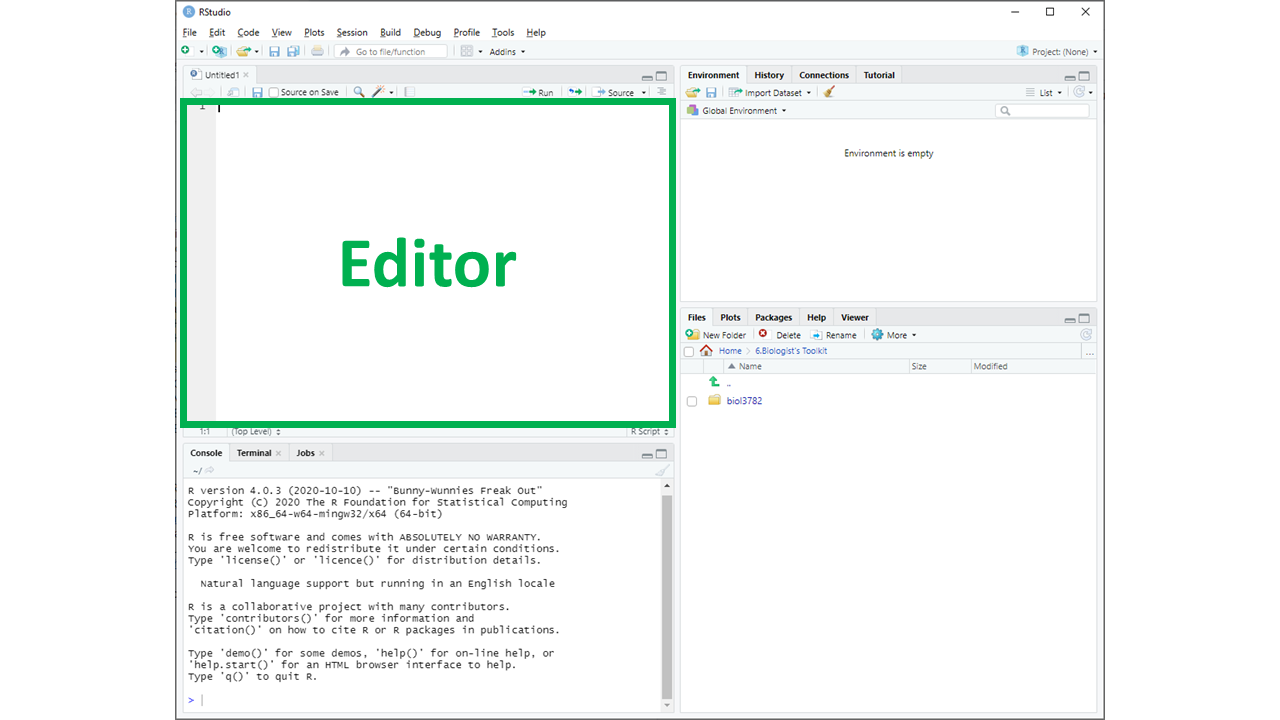
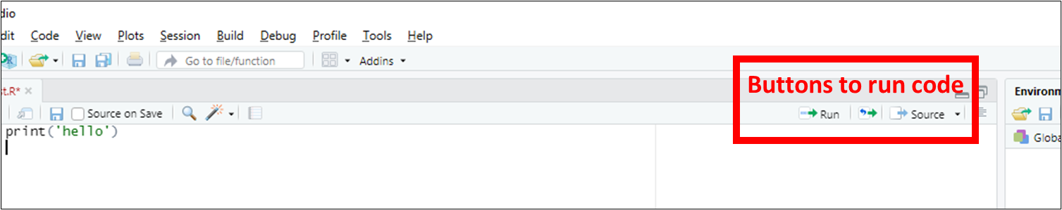
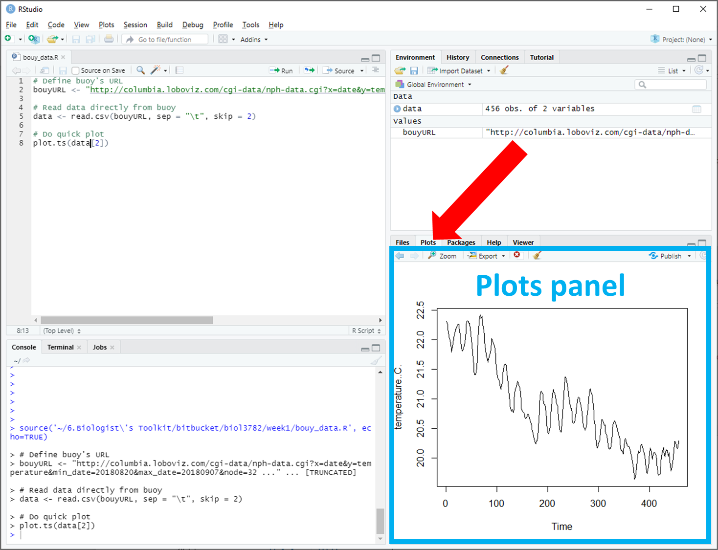
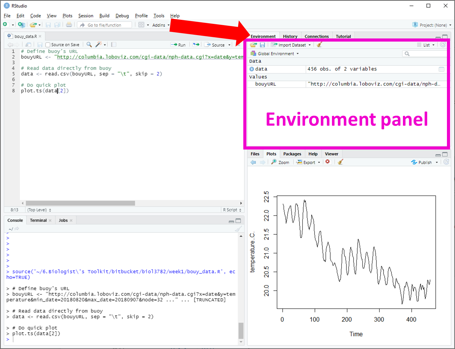
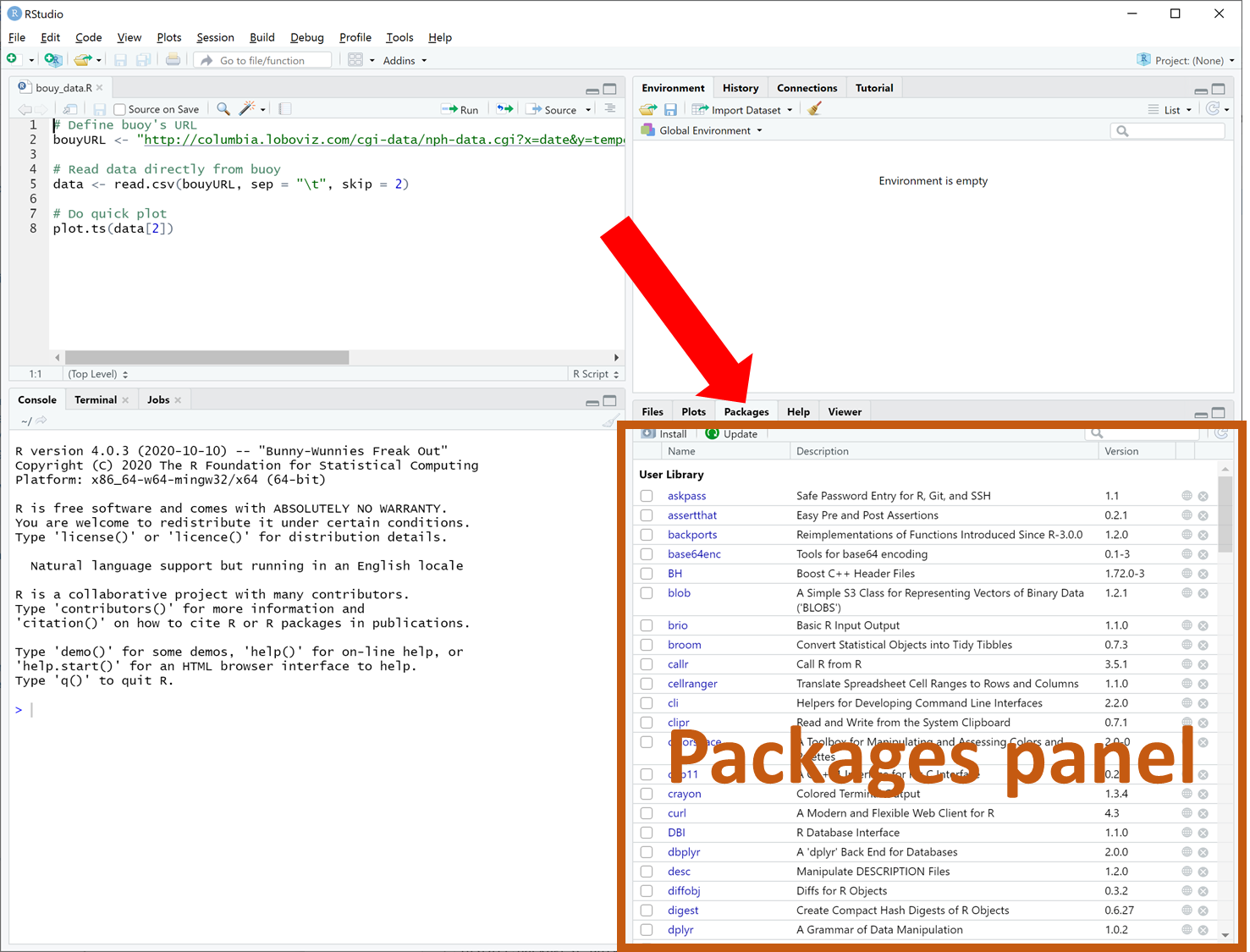
3. RStudio: This is the main program where you will use to write and run R code. We'll talk more about RStudio below.

Work flow in a typical Lab

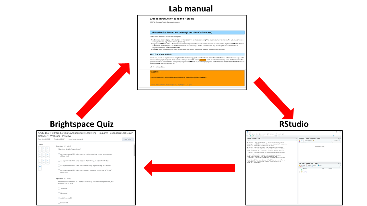
In most labs, you will be required to read along the Lab manual and copy-paste code from the lab manual into RStudio to run it. This will create output in the form of numbers, graphs, maps, etc. Occasionally, you will need to answer questions, which are written inside orange boxes like the one below. The questions need to be answered in the corresponding Brightspace LAB Questions. So, you will be jumping back and forth between the Lab manual, RStudio and the Brightspace LAB Questions throughout the lab.

Let's do a test question...

Sample question: Can you see THIS question in your Brightspace LAB quiz?

Where is my code?

Data, code and the results produced by the code can be stored in many places, including:

1. "The cloud" (e.g. BrightSpace, your OneDrive, GitHub, a website, etc.)
2. Your "physical" computer (like the computer that you are working on at this moment). Within your computer, data and code can be stored:
   • in the hard-drive,
   • in memory and
   • on the screen

Note that:

• Computers can ONLY see and work with code and data stored in memory
• Humans can ONLY see code and data shown on the screen
• When turning your computer off, code/data in both the memory and the screen are lost forever! Therefore, make sure that you save your work on your hard-drive or the cloud, before turning your computer off.

We will see below how to move code (and data) between all these storage areas (i.e. memory, hard-drive, screen, cloud). keeping track of where is your code/data stored, is one of the most common sources of errors during coding.

R

'R' is the most commonly used programming language among biologists today, primarily due to its object-oriented syntax and its powerful statistical and graphics capabilities. R was preinstalled in all Lab computers; however, if you want to follow along in your own laptop, you can install R directly from https://www.r-project.org

Note that when you installed R, a lot of code was copied from "The Cloud" into your hard-drive, in a location that we will call "the R Directory". The actual location of "the R Directory" is not important to us in this course. However, if you are curious and try to find it, just make sure that you DO NOT move, delete or add anything within "the R Directory"! You can break R's proper functioning.

Micro-introduction to coding in R

Code of any programing language is made by a mixture of variables, functions, arguments, comments, data, packages, operators and a few other "objects". Learning any specific programming language entails to learn the specific "syntax" on how to work with these different types of "objects".

In this first lab, your job will be to learn to tell apart all these different types of "objects". Below are pointers to help you:

Object type	What do they do?	How to spot them?
Variables	They store data or other objects	They are ALWAYS made by the user (i.e. you) using the "arrow operator" (i.e. <-). Example: In y <- 9702... y is a variable Following the example above, pretend that a few lines down the y <- 9702 code you find the following stament: print(y) Now you are wondering if the y in print(y) is a variable or not. To solve this, you may have to read the code above to see if you find a statement that declares (i.e. makes) the variable, in this case y <- 9702. In other words, sometimes you have to quickly read the code ABOVE a "statement of interest" to see which parts are variables.
Functions	This is how R does its magic! They are "commands" that come included in R, and that do things like calculate means, make graphs, do stats, etc.	Functions follow one the syntaxes below. Note that parentheses ( ) ALWAYS accompany functions: FunctionName() FunctionName(arguments) Function.Name(arguments) Example: In print(y)... print is a function
Arguments	They are instructions to guide the function on how to do their task properly.	They are always inside the parentheses of a function (technically, input is also an argument). Note that Variables are often placed inside the parentheses of a Function to be used as Arguments of the Function. Example: In print("Hello World")... "Hello World" is a argument
Packages	Packages or Libraries are a collection of additional Functions that you can install, load and use along with the R-included functions.	They are loaded using the syntax library(PackageName). Example: In library(ggplot2)... ggplot2 is a package
Comments	They are lines meant for human-eyes-only and thus are ignored by R	Comments lines ALWAYS start with a hashtag # Example: In y <- 9702 # this is a new variable ... # this is a new variable is a comment
Data	These are numbers or letters.	These are numbers or letters surrounded by quotes " ". Note that Data can be placed inside the parentheses of a Function to be used as Arguments of the Function. Example: In y <- 9702... 9702 is data

Take a look at the code below and see if you can figure out what are the different "objects" used in this code... when you are done, you can take a look at the answer below.

Consider the following R code, which prints-to-screen 9 and "Hello World":

# Lets do some variables
x <- 9
my_var <- "Hello World"

# Now, lets print the variables to screen
print(x)
print(my_var)

[1] 9
[1] "Hello World"

---

ANSWER:

• # Lets do some variables is a comment (in line 1)
• x and my_var are variables (created in lines 2 and 3)
• # Now, lets print the variables to screen is a comment (in line 5)
• 9 and "Hello World" are data (in lines 2 and 3)
• print is a function (same function in lines 6 and 7)
• The x in print(x) is an Argument of the print function (in line 6). Note that x is also a variable (made in line 2)
• The my_var in print(my_var) is an Argument of the print function (in line 6). Note that my_var is also a variable (made in line 3)

---

Consider the following R code:

# Lets do a variable
ThisIsMyVariable <- 39878

# Lets query all the variables currently loaded in Memory
ls()

1. 'my_var'
2. 'ThisIsMyVariable'
3. 'x'

What is:

ThisIsMyVariable

What is:

ls

What is:

39878

RStudio

Most people do "coding" (in any language) using an "Integrated Development Environment" (IDE), which are programs designed to make "coding" easier. IDE's make it easier to run your code, get help, manage multiple projects and files, color-code your code as you write it, etc. IDE's are like a swiss-army-knife for coding. Many IDE's are free. Take a look at this list of IDE's

RStudio is a free IDE especially designed to work with R. RStudio was also pre-installed in all Lab computers; however, if you want to follow along in your own laptop, you can install RStudio directly from https://rstudio.com/

• To open RStudio, search in the taskbar for "RStudio", the program looks as follows:

Note that when you open RStudio, behind the scenes a bunch of code was loaded into memory from "the R Directory" (i.e. hard-drive).

The RStudio screen is divided in multiple panels. We will review the most important panels next.

RStudio's "Console"

The is a live instance of R. It is the most direct way to connect your computer's memory (i.e. where R is loaded) to your screen. This is the place where R will display error messages, warnings, and some code output. The is also where you can quickly interact with R by writing code and then clicking [Enter] When you click [Enter], anything you wrote on the will be loaded to memory and executed immediately. Let's try it:

Type the following code in the , then press [Enter]

print('hello world!')

[1] "hello world!"

After you typed:

print('hello world!')
What got displayed on the screen?

You can also use R's console as a simple calculator.

Type the following code in the , then press [Enter]

14 + 9

23

Again, it is important to note that when you clicked [Enter], anything you wrote on the was loaded to memory and executed immediately.

RStudio's Help panel

As we said above, most of the "magic" done in R is done through functions (e.g. calculate means, standard deviations, make graphs, print maps, etc.). Each function has specific instructions on how to use it, what arguments it needs, what kind of inputs it requires, etc. Luckily, the instruction manual of every function in R is accessible via the Help panel. To access it simple chick on the Help tab; and to use it simply type the name of the function in the search bar within the Help panel.

Another way to display the function's instruction manual in the Help panel is by typing in the the function name preceded by a ?. For example:

?print

...or you can use the help() function. For example:

help(print)

The instruction manual of a function is broken down into sections:

• Description: An extended description of what the function does.
• Usage: The arguments of the function and their default values.
• Arguments: An explanation of the data each argument is expecting.
• Details: Any important details to be aware of.
• Value: The data the function returns.
• See Also: Any related functions you might find useful.
• Examples: Some examples for how to use the function.

Different functions might have different sections, but these are the main ones you should be aware of.

From within the function help page, you can highlight code in the Examples and hit Ctrl+Return to run it in RStudio console. This gives you a quick way to get a feel for how a function works.

Other ways to get help

• Google your question followed by R
  • Note that Google Results from Stack overflow are usually high quality answers
• Search using https://rseek.org/
• Search directly in Stack Overflow within the [r] tag

Other ports of call:

• Quick R
• RStudio cheat sheets
• Cookbook for R

RStudio's "Editor"

To be able to see the , you need to have an "R script" file open. If you don't have any file open, you have to create a new one by clicking on the "green plus sign" and selecting "R script" (see below):

The is the space where you write your code so that you can execute it later. The is shown below inside the green box.

The is just a text editor like Notepad (in Windows) or TextEdit (in Mac). However, note that RStudio's color-codes your text so that it can be read with ease. It will also perform some basic quality control and will tell you if you made a mistake (more on this later).

If you haven't open a new R script file, follow instructions above to create one, and then type the code below in the :

print('Hello world!')

[1] "Hello world!"

Great! Now it is time to your script!

Running your code

There are many ways to run the code you wrote in the editor. They require you to click on one the "run" buttons or use the keyboard shortcuts (see below).

Executing a Single Line

To execute the line of code where the cursor currently resides, you need to press the Ctrl+Enter keyboard shortcut (or use the "Run single line" button in the "Run toolbar").

After executing the line of code, RStudio automatically advances the cursor to the next line. This enables you to single-step through a sequence of lines.

Executing Multiple Lines

There are three ways to execute multiple lines from within the editor:

• Select the lines and press the Ctrl+Enter keyboard shortcut (or use the button in the "Run toolbar"); or
• After executing a selection of code, use the Re-Run Previous Region command (or its associated toolbar button) to run the same selection again. Note that changes to the selection including additional, removal, and modification of lines will be reflected in this subsequent run of the selection.
• To run the entire document, press the Ctrl+Shift+Enter keyboard shortcut (or use the toolbar button).

When you click the or buttons, RStudio automatically loads the code from the Screen (i.e. the Editor) into memory for execution.

Let's do a test.

Run your script (i.e. the one you made in the task above), by clicking in the button . If your script ran properly, you should be able to "Hello world!" in the .

Try running your code with all the buttons and keyboard shortcuts explained above.

As you see, every time you run the code in the , the output is displayed in the

After you write some code in the Editor, what happens when you click the "source" button?

RStudio's "Working Directory"

The working directory is the location in your computer where RStudio is reading and writing files. If you click on the Files tab, you likely will be viewing the working directory and its contents. Also, within the Files tab, you can click on the More button to "Set the working directory" or "Go to the Working Directory".

The location displayed in the Files tab is not always the working directory. Therefore, the best way to get the working directory, is to use the getwd() function, see task below.

Type in the the following line and click [Enter].

getwd()

'C:/Users/Diego/Documents/6.Biologist\'s Toolkit/biol3782/week1'

• Did you see get the working directory?

• Did it match the location shown in the Files tab.

---

When you are working on a lab that requires ancillary data files or ancillary R code files, you need to make sure these files are in the working directory. You can download them directly to the working directory, or you can change the working directory to be folder where you downloaded your files.

Changing the "Working directory"

To change the working directory, you can:

• Use the setwd() function.

...or you can:

• (1) go to the Files tab, (2) navigate to the folder that you want to make your new working directory, (3) click on the "More" button, and (4) select Set As Working Directory

You are starting to work on a lab that requires 2 ancillary data files and 3 ancillary R code files. You download all these files from BrightSpace into you Laptop. Which of the following describes best what happened to the data/code?

You are starting to work on a lab that requires 2 ancillary data files and 3 ancillary R script files. Where in your laptop do you have to put these files?

Saving your code

To save your file to your hard-drive, simply click the "Save" button on the Editor (it looks like a floppy disk). You can name your file anything you want, but the extension will be automatically set as .R, which is the default extension for R files.

After you write some code in the Editor, clicking the "save" button technically transfers code from the Screen (i.e. the Editor) into a file in your hard-drive.

Save the R script file you created earlier. Name it hello_world.R

After you write some code in the Editor, what happens when you click the "save" button?

Real-life Example #1: Downloading real-time data from an oceanographic buoy in Oregon

To explain the Plots and Environment panels in RStudio, it is required that we load some data and make a plot. This is a nice opportunity to do some real-life data mining and visualization. Let's download data from a buoy in Oregon. USA.

There is an autonomous buoy in the Columbia River (Oregon, USA) that broadcasts real-time ocean data via the following server: http://columbia.loboviz.com/

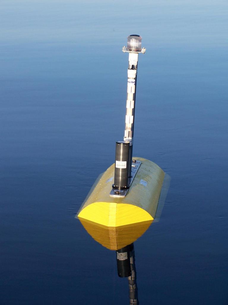LOBO Buoy

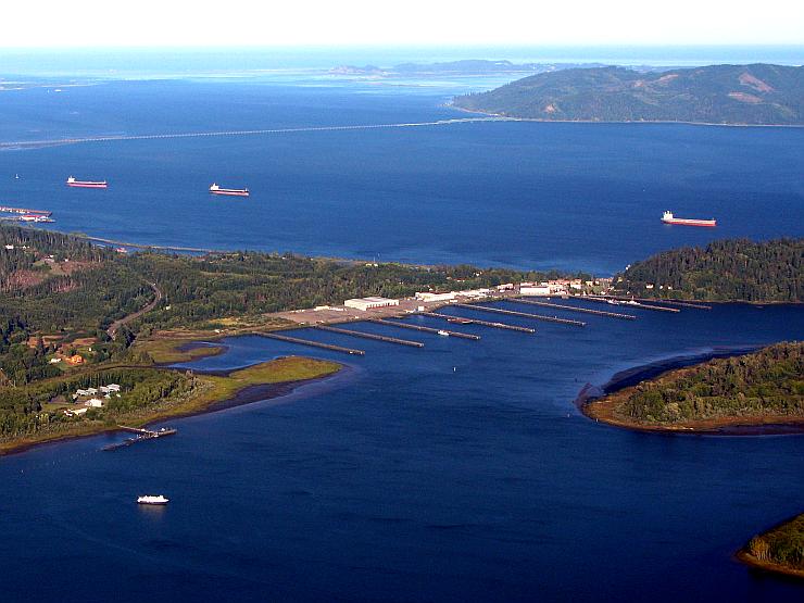Columbia River (Oregon, USA)

The following code connects to the buoy's server, downloads data, and makes a simple plot. Note that A LOT gets done with just 3 lines of code. This is the magic of "coding"!

In RStudio's open a new file and save it as buoy.R. Copy-paste the code below to your new file and click

# Define buoy's URL
bouyURL <- "https://raw.githubusercontent.com/Diego-Ibarra/biol3782/main/week1/data/buoy_data.csv" # http://columbia.loboviz.com/ is down at the moment. Redirect to saved .csv file in course's repo

# Read data directly from buoy
data <- read.csv(bouyURL, sep = ",")

# Do quick plot
plot.ts(data[3])

In this simple graph, the time x-axis is in not displayed as dates, but instead as "record number". Therefore, we do not know if this time-series spans a few weeks or a few decades. However, we can probably deduce that the time span by looking at the y-axis. If the time-series span a few decades, you should see high temperatures of around 25 °C (maximum in the summer) and low temperatures around 5 or 10 °C (minimum in the winter). We do not see that range in the y-axis. Therefore, I think the time-series spans only a few weeks in late summer or early fall, because the temperature starts high (approx. 22 °C) and decrease a couple of degrees (~20 °C) over the span of the series. While Oregon is not a cold as Halifax, the water surface in the Columbia River should decrease in winter to just 5 or 10 °C, which we do not see in the plot. The high frequency variability (the up and down "wiggles" in temperature) is likely due to day-night temperature fluctuations in air temperature, or ebb-flood tide fluctuations. All that from 3 lines of code!

From the code above, in line 2... What is:

bouyURL

From the code above, in line 5... What is:

data

From the code above, in line 5... What is:

read.csv

From the code above, in line 5... What are:

bouyURL, sep = "\t", skip = 2

From the code above, in line 7... What is:

# Do quick plot

From the code above, in line 8... What is:

plot.ts

From the code above, in line 2... What is:

"http://columbia.loboviz.com/cgi-data/nph-data.cgi?x=date&y=temperature&min_date=20180820&max_date=20180907&node=32&data_format=text"

From the code above, in line 1... What is:

# Define buoy's URL

RStudio's "Plots" panel

After you ran buoy.R, you will see the plot above in your RStudio's "Plots" panel (see below).

RStudio's "Environment" panel

After you ran buoy.R, you will see the variables you created (i.e. bouyURL and data) in the "Environment panel" (see below).

After you ran buoy.R and clicked , R read the code you wrote on the editor, created the bouyURL and data variables in memory, and sent their name and value to the screen (in the Environment panel). Again, all that with the click of a button!

R Packages (or Libraries)

As said above, packages (also called libraries) are collections of functions, made by "community members", that you can download and use for free. Note that there are two steps required before you can use a package:

1. First, you have to "Install" the package. In this step, the package's code is downloaded from "the cloud" and saved into your computer's hard-drive. This step needs to be done once for every new installation of R; if you buy a new computer and install a R for the first time, you will need to install the packages you want to use.

   • To "Install" a package, use the function: install()
   • For example: install(ggplot2)
   • You can also install new packages using the install button in the Packages panel (see below)
     
     

2. Then, you have to load the package. In this step, the package's code is loaded from your hard-drive into your computer's memory. This step needs to be done once every time R is "turned on".

   • To "load" a package, use the function: library()
   • For example: library(ggplot2)

To see a list of all available R packages, see: https://cran.r-project.org/web/packages/available_packages_by_name.html

RStudio's Packages panel

To see RStudio's Packages panel, click on the Packages tab. In RStudio's Packages panel, you can see a list of installed packages (see image below). Note that the packages that are currently loaded into memory are shown with a "tick" besides their package name.

Real-life Example #2: Downloading real-time data from a Glider in Nova Scotia

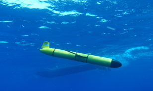Slocum Glider

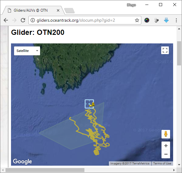Current deployment

Autonomous Underwater Vehicles (AUV's) or "gliders", are robots programed by scientist to autonomously navigate a pre-programmed transect while collecting an assortment of data, from water temperature, to phytoplankton fluorescence, to whale calls. Dalhousie University and the Ocean Tracking Network have a fleet of gliders that patrol Nova Scotia waters.

The code below pulls data from a glider deployed off the coast of Nova Scotia (http://ceotr.ocean.dal.ca/gliders/). The code plots a rough depth-vs-time scatter plot.

If you do not have already installed ggplot2 and viridis, copy paste the following code to RStudio's and click [Enter]:

install.packages("ggplot2")
install.packages("viridis")

package 'ggplot2' successfully unpacked and MD5 sums checked

The downloaded binary packages are in
	C:\Users\Diego\AppData\Local\Temp\RtmpOq3avG\downloaded_packages
package 'viridis' successfully unpacked and MD5 sums checked

The downloaded binary packages are in
	C:\Users\Diego\AppData\Local\Temp\RtmpOq3avG\downloaded_packages

Then...

In RStudio, open a new file, name it glider.R, copy-paste the code below in the , and click ...note that it takes a bit of time to finish running.

# Import library
library(ggplot2)
library(viridis)

# Define URL for OTN glider
URL = 'http://gliders.oceantrack.org/data/live/bond_sci_water_temp_live.csv'

# Read data directly from buoy
data <- read.csv(URL, sep = ",")

# Set plots to be drawn with a resonable size
options(repr.plot.width=8, repr.plot.height=4)

# Scatter plot
# Assign plot to a variable "sp"
sp <- ggplot(data, aes(x=unixtime, y=depth, color=sci_water_temp))

# Draw the plot
sp + geom_point() + 
     scale_y_reverse() +
     scale_color_viridis(limits = c(5,20), option="plasma")

Warning message:
"package 'ggplot2' was built under R version 3.6.3"Warning message:
"package 'viridis' was built under R version 3.6.3"Loading required package: viridisLite

From the code above, in line 1... What is:

# Import library

From the code above, in line 3... What is:

viridis

From the code above, in line 6... What is:

URL

From the code above, in line 6... What is:

'http://gliders.oceantrack.org/data/live/bond_sci_water_temp_live.csv'

From the code above, in line 9... What are:

URL, sep = ","

From the code above, in line 9... What is:

data

From the code above, in line 9... What is:

read.csv

From the code above, in line 16... What is:

sp

From the code above, in line 18... What is:

# Draw the plot

From the code above, in line 20... What is:

scale_y_reverse

From the code above, in line 21... What is:

scale_color_viridis

From the code above, in line 21... What are:

limits = c(5,20), option="plasma"

From the code above, in line 19... What is:

sp

From the code above, in line 2... What is:

ggplot2

Real-life Example #3: Downloading Satellite data from an ERDDAP server

In this real-life case study, we will use an ERDDAP data server to download Sea Surface Temperature data from the Nova Scotia Region.

ERDDAP is a data server that simplifies the download of subsets of scientific datasets to make graphs and maps, and other analyses.

Many universities and government agencies use ERDDAP. Here we will be using one of NOAA's ERDDAP: https://coastwatch.pfeg.noaa.gov/erddap/info/index.html?page=1&itemsPerPage=2000

---

First, lets get ourselves some Sea Surface Temperature (SST) from the Nova Scotia region. For this we will use an ERDDAP product consisting on averages of several satellites, including AVHRR, AATSR, SEVIRI, AMSRE, TMI and others.

In RStudio's open a new file and save it as satellite.R. Copy-paste the code below and click ...note that it takes a bit of time to finish running.

# Define ERDDAP's URL
URL <- "https://coastwatch.pfeg.noaa.gov/erddap/griddap/jplUKMO_OSTIAv20.csv?analysed_sst%5B(2020-12-22T12:00:00Z):1:(2020-12-22T12:00:00Z)%5D%5B(41.025):1:(52.025)%5D%5B(-67.975):1:(-54.675)%5D"

# Read data from ERDDAP
data <- read.csv(URL, sep = ",", skip = 1)

# -- Rough heatmap ----
# Assign plot to a variable "hm"
hm <- ggplot(data, aes(degrees_east, degrees_north, fill= degree_C)) + 
  geom_tile()

# Draw the plot
hm + scale_fill_viridis(discrete=FALSE)

From the code above, in line 1... What is:

# Define ERDDAP's URL

From the code above, in line 2... What is:

URL

From the code above, in line 2... What is:

"https://coastwatch.pfeg.noaa.gov/erddap/griddap/jplUKMO_OSTIAv20.csv?analysed_sst%5B(2020-12-22T12:00:00Z):1:(2020-12-22T12:00:00Z)%5D%5B(41.025):1:(52.025)%5D%5B(-67.975):1:(-54.675)%5D"

From the code above, in line 5... What is:

data

From the code above, in line 5... What is:

read.csv

From the code above, in line 5... What are:

URL, sep = ",", skip = 1

From the code above, in line 9... What is:

hm

From the code above, in line 9... What is:

ggplot

From the code above, in line 9... What is:

data, aes(degrees_east, degrees_north, fill= degree_C)

From the code above, in line 13... What is:

discrete=FALSE

From the code above, in line 13... What is:

scale_fill_viridis

From the code above, in line 13... What is:

hm

In RStudio's , copy-paste the code below at the bottom of satellite.R. Select the newly pasted code and and click

# -- Better heatmap (projected)----
# Assign plot to a variable "hm"
hm <- ggplot(data, aes(degrees_east, degrees_north, fill= degree_C)) + 
  geom_tile()

# Draw the plot
hm + scale_fill_viridis(discrete=FALSE, option="plasma") + # Add "plasma" colormap 
     borders("world", fill="grey90",colour="#8c8c8c") +  # Add continents and coastlines
     coord_fixed(xlim = c(-68, -55),ylim = c(41, 52)) # Add projection and set map limits

If everything went well, the image plot above should have appeared in your RStudio's "Plot panel". As you can see, it is a projected map with nicer land and coastlines than the plot made in the previous task. You should be able to see that in the Lawrence River and Gulf of St Lawrence there is cold water of around 3°C. However, south from Nova Scotia there is water of about 20°C; this is the Gulf Stream, which is a warm-water current formed in the Gulf of Mexico and that runs all the way into Ireland.

From the code above, in line 8... What is:

borders

From the code above, in line 8... What do you think the following do?

borders("world", fill="grey90",colour="#8c8c8c")

From the heatmap above... There is a mass of warm water around -64°E and 42°N. What do you think is the source of such warm water?

---

Some parts of this lab where borrowed from:

• Software Carpentry
• Data Carpentry
• Spatial Data Science with R

This is the end of lab

---

---

Code below is for formatting of this lab. Do not alter!

cssFile <- '../css/custom.css'
IRdisplay::display_html(readChar(cssFile, file.info(cssFile)$size))

IRdisplay::display_html("<style>.Q::before {counter-increment: question_num;
    content: 'QUESTION ' counter(question_num) ': '; white-space: pre; }.T::before {counter-increment: task_num;
    content: 'Task ' counter(task_num) ': ';</style>")